Excel tutorials

Sometimes it is good to highlight specific words or sentences in Excel to make the user aware of something specific. It can be a specific group or ID for example.

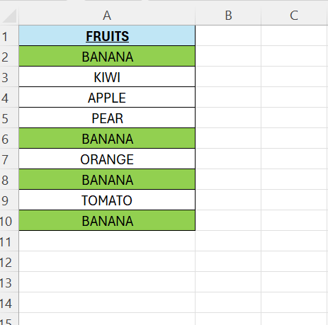
Below we have a list of fruits in Column A, we want to highlight all the cells that contain the word “BANANA”.

To make this work, we will use two functions in combination. The functions are =ISNUMBER() and =SEARCH(). We are going to enter the formula under “Conditional Formatting”.

Lets break down the formula first to see how it is going to work.

For the SEARCH part: enter the next in cell D2:

=IFERROR(SEARCH(“BANANA”;A2);””)

We search for our keyword “BANANA” in cell A2. If we get a match, the returned value is 1. Otherwise, we return empty.

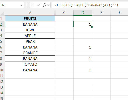
If we drag the formula down, we can see a pattern. We get 1 in 4 cells. That shows where our keyword is available in column A.

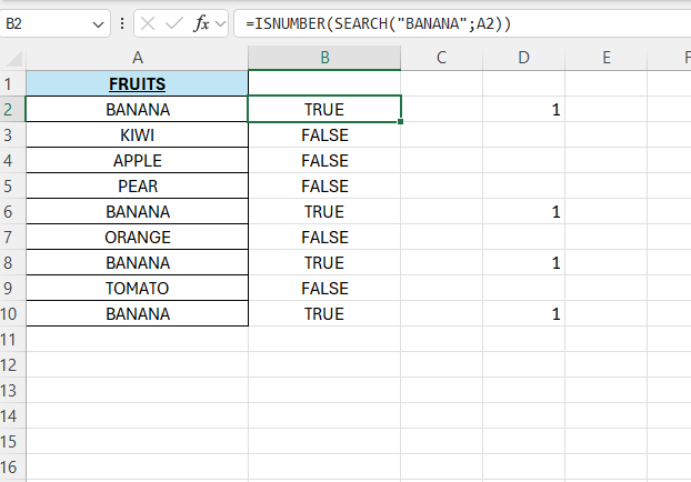
The next part is the ISNUMBER-part. This operation returns TRUE or FALSE. It depends on whether it is a number or not.

In B2, enter the below:

=ISNUMBER(SEARCH(“BANANA”;A2))

Now, we can delete what we have done in column B and D. Select the cells A2:A10 in column A, then go to “Conditional Formatting”. Select “New Rule” and then “Use a formula to determine which cells to format”.

Then enter our formula in the formula field:

=ISNUMBER(SEARCH(“BANANA”;A2))

Then click “Format” – choose the “Fill” and choose a color, then click OK and OK again.

Final result