Excel tutorials

Let’s say the user is required to enter a 5-digit number, one way to assure this is to use data validation.

In this post we also have a bunch of numbers the user is not allowed to enter, an exclusion list.

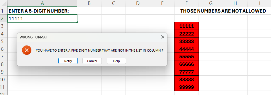
The user are supposed to enter the numbers in column A, the exclusion list is present in column F. If the user enters one of those, we get a warning, as we can see in the picture above.

Follow the steps outlined below to set this up.

1. Select the cells in column A that you want to apply data validation to
2. Go to the Data tab, select “Data Validation”
3. In the “Settings” tab – under “Allow” -> choose “Custom”
4. In the “Formula” bar -> enter the formula:
5. =AND(ISNUMBER(A2);LEN(A2)=5;COUNTIF($F$3:$F$11;A2)=0)

This states that A2 have to be a number, the length have to be 5, and it must not be equal to any of the values in F2:F11.