Excel tutorials

In the previous part we calculated work ours between two times, but often we have to include a lunch break.

• Format columns A to D as Time
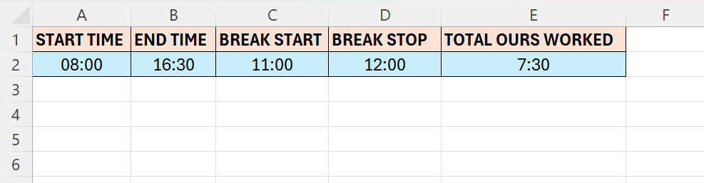
• In cell E2 we are going to enter our formula
• The formula cell will have a Custom formatting
• [t]:mm
• The formula is rather the same as in the last tutorial, we just have to take the lunch into consideration
• The complete formula looks like below
• ((B2-A2)-(D2-C2))