Excel tutorials

A common task in Excel is to compare columns and find missing values in one of them

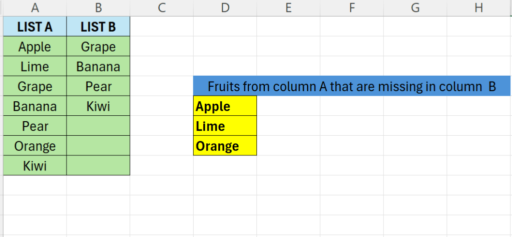
Above we have two lists. The goal is to find the fruits in List A that are missing from List B.

• First we will use the VLOOKUP function
• =VLOOKUP(A2:A8;B2:B5;1;FALSE)
• Above tries to look up all the values from List A in List B
• The result will be a list of fruits that exists, the other will be represented as #N/A
• We will wrap the above formula in ISNA
• This checks if a cell contains #N/A – returning TRUE if it does, FALSE otherwise
• Now we can use the FILTER together with ISNA to filter the fruits from LIST A that had a value of #N/A
• =FILTER(A2:A8;ISNA(VLOOKUP(A2:A8;B2:B5;1;FALSE)))