Excel tutorials

In the previous post we saw how we can use SUMPRODUCT to calculate products. Another feature of this function is that it allows us to specify a calculation on just part of a column. For example, only IDs that start with 123.

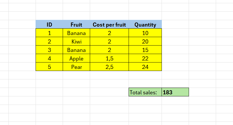
In the previous post we calculated the total sales for all the fruits in the list below.

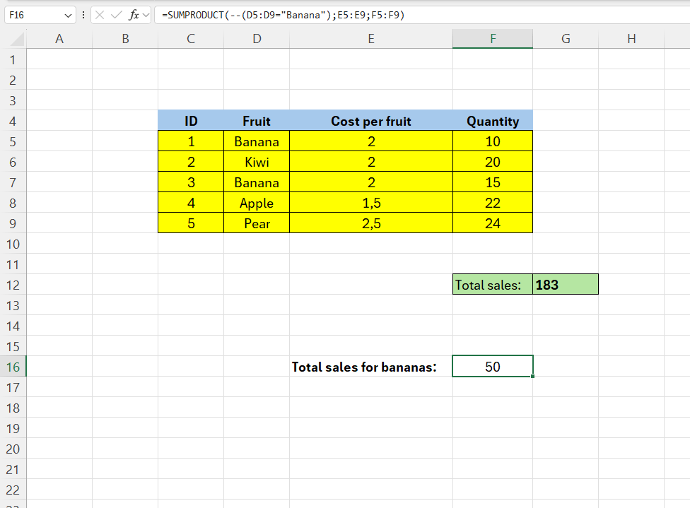
What if we only wanted to calculate the sales for Bananas only? SUMPRODUCT can only handle numerical values. We need a way to convert the array of TRUE and FALSE into 1s and 0s. For this, we use the double negative.

In F16 – enter the following formula:

=SUMPRODUCT(–(D5:D9=”Banana”);E5:E9;F5:F9)

Here we set that the value to look for should be “Banana” – the rest is the same as in the last post.