Excel tutorials

A common task in Excel is to spot differences between list or compare them in some way. Here we are going to highlight values that are missing in one list. There are multiple ways to do this – here we are going to use conditional formatting.

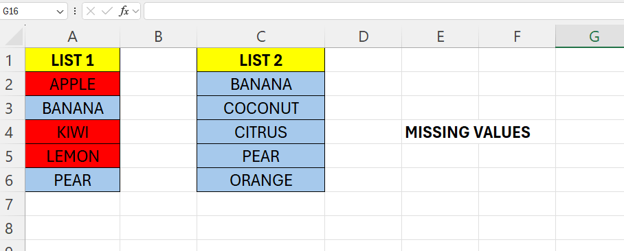
Above we have two lists with some names in it, the goal here is to check which values in list 1 that are NOT present in List 2.

Start by selecting the range A2:A6 – then go to “Conditional Formatting” and choose “New Rule…”.

We are going to make use of the =COUNTIF() function to achieve this. This method returns the number of times a value appears in a selection. When a value is not found, the function will return 0 – this is how we trigger our conditional formatting.

Enter the formula in the formula field:

=COUNTIF($C$2:$C$6;A2)=0

Then select “Format” and choose a color for the formatting.

Now, the values in red are those not found in List 2.