Excel tutorials

In Excel we often want to search for a specific item or value, when that specific value does not exist, we want to get a notification about that.

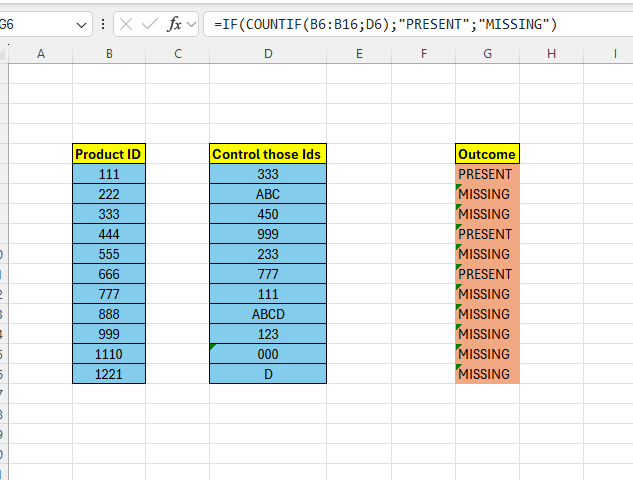
Above we have a bunch of IDs in column B, in column D we have another bunch of IDs that we want to check if they are present in column B or not.

One way to do it is to represent present values with 1, missing values with 0.

In G6 enter the below formula:

=COUNTIF(B6:B16;D6)

This is actually it, but lets make it a little more user-friendly.

We can use the =IF() to output a text for missing/present values instead of representing them with 1 or 0.

Enter the below formula in G6:

=IF(COUNTIF(B6:B16;D6);”PRESENT”;”MISSING”)