Excel tutorials

When we are using VLOOKUP to find a value, and Excel cannot find the value, it usually returns #N/A

We can use different ways to catch this error and return any value. As in our previous post we are going to use =IFERROR()

Lets play with some example-data

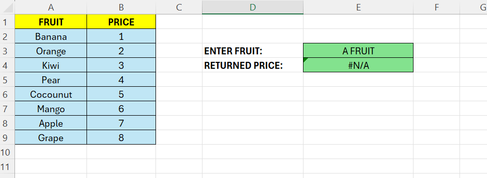
Above we have some fruits in column A, and its price in column B. We want to enter a name of a fruit in E3 and get its price in E4. As we can see above, “A FRUIT” does not exist in column A – so we get a #N/A

The basic formula in E4 is as below:

=VLOOKUP(E3;A2:B9;2;FALSE)

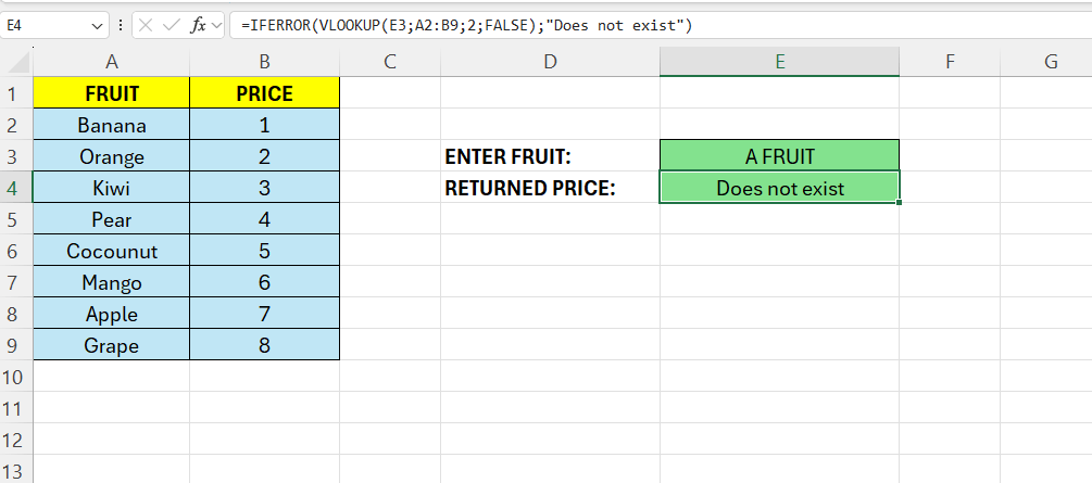
To display something more meaningful, for example “Does not exist”, we need to extend the formula above with the =IFERROR() function.

The complete formula then look like this:

=IFERROR(VLOOKUP(E3;A2:B9;2;FALSE);”Does not exist”)