Excel tutorials

In this tutorial we are going to see how we can extract the first digit in i string.

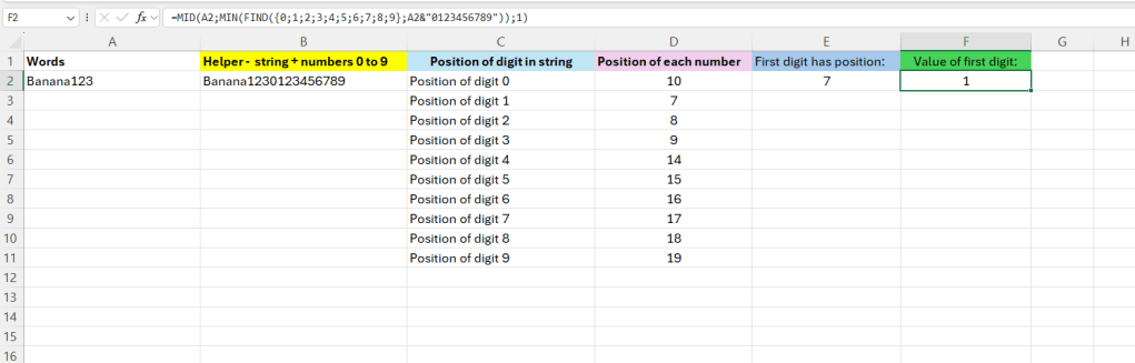
Below we have an example. In A2 we have a word with some digits in it – the goal here is to extract the first digit in it – that is number 1 in this case.

We are going to make this in parts – first we are going to create a textstring in column B. This will contain the word in A2 + the digits 0 to 9.

Formula in B2:

=A2&”0123456789″

We are going to make use of array-formulas later on – for clarification in column D – I have included the position of each number in the textstring.

To calculate the position we are going to use the =FIND() function.

Enter the following in D2:

=FIND({0;1;2;3;4;5;6;7;8;9};A2&”0123456789″)

Just press enter now – then we can see the positions. Digit 0 is at position 10, digit 1 is at position 7 and so on.

We are only interested in the first digit in the string in A2 – so we can use =MIN() to get the smallest number from column D – we can see that it is 7, position 7 that is.

Formula in E2:

=MIN(FIND({0;1;2;3;4;5;6;7;8;9};A2&”0123456789″))

Now to get the value itself, we can use the =MID() function

=MID(A2;7;1) (7 is from E2, 1 is the number of characters we want to get)

A more correct way is to include MID into the function:

=MID(A2;MIN(FIND({0;1;2;3;4;5;6;7;8;9};A2&”0123456789″));1)

Normally when you enter the formula in D2 – dont hit ENTER, use CTRL+SHIFT+ENTER – that is because it is a so called array-formula iterating over the numbers.