Excel tutorials

One of the more common functions for looking up values is to combine =INDEX() with =MATCH()

Below we have a list of fruits, price and weight and color. We want to enter a fruit – then Excel should fetch the price for us.

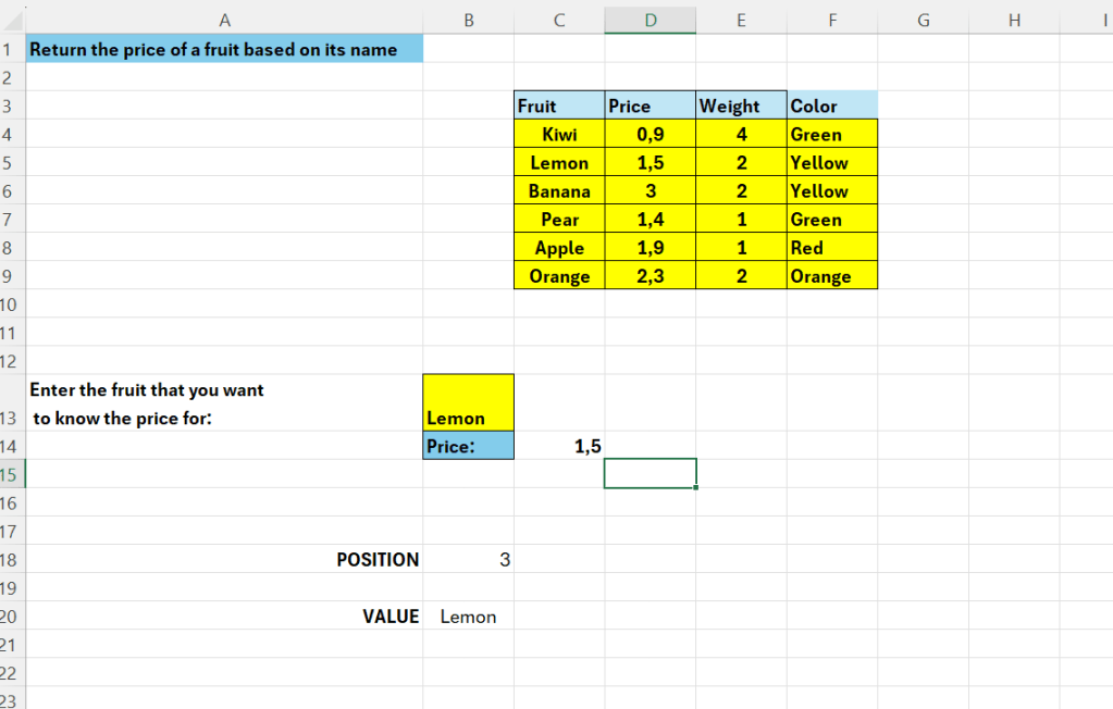
In B13 we enter a fruit that we want Excel to look-up for us- and in C14 – the price will show.

We can make the formula in chunks – first we can get the value using =INDEX()

=INDEX(C3:C9;B18;1)

This will give us the fruit – Lemon

The above searches in the range C3:C9, we supply the row_number – which is the value in B18 – which is 1

We use =MATCH() to look up this value

=MATCH(B13;C3:C9;0)

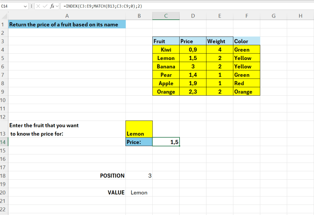
Then we can combine this in C14:

=INDEX(C3:E9;MATCH(B13;C3:C9;0);2)

The digit 2 at the end, is the column to search in – the column “Price”