Excel tutorials

If we have one or more lists in Excel – sometimes we need to extract duplicates from those lists.

To achieve this we need to use multiple functions. In this example we are going to use the =FILTER() and =COUNTIF() functions.

Below we have some example data in Column A – in column B a helper-column we will look into below, in Column C we have our duplicates – we will filter the distinct values out from this later on in this tutorial.

We start with the =COUNTIF() function in cell B2.

=COUNTIF(A2:A10;A2:A10)

This counts cells based on a condition or criteria, this allows us to get the duplicate values. Above if a value is 1 – it is not a duplicate

We can change the above formula to this:

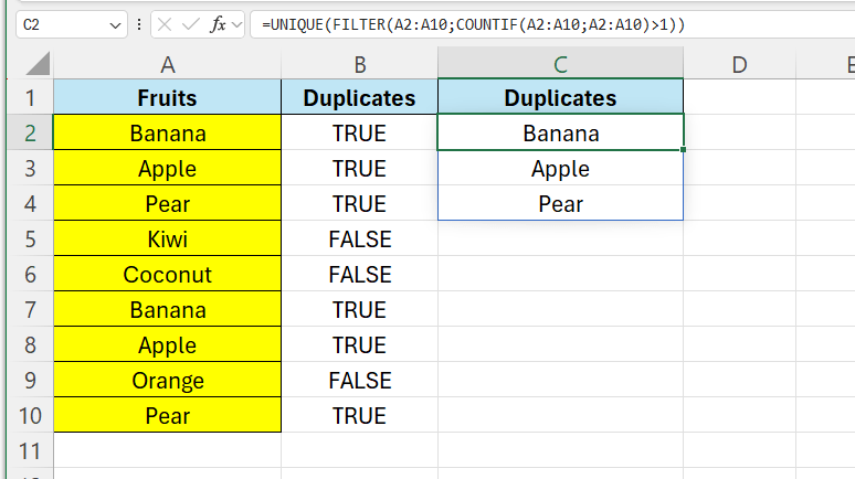
=COUNTIF(A2:A10;A2:A10)>1

Now we will get a TRUE or FALSE instead – TRUE if it is a duplicate – false otherwise.

Next we will use =FILTER() to extract values based on the condition from the =COUNTIF() function.

In C2 enter the following formula:

=FILTER(A2:A10;COUNTIF(A2:A10;A2:A10)>1)

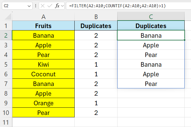
As we can see, the duplicates appear more than 1 time here as well, to get rid of those, we can use the =UNIQUE() function.