Excel tutorials

In the last 2 post we have seen how we can use VLOOKUP to retrieve values for us. Those examples go

t information from the same sheet. In this part we are going to see how we can access data from another sheet in Excel.

Enter the following data in Sheet1:

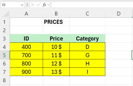
Enter the following data in Sheet2:

Our mission here is to fill column C in Sheet1 with data.

In Cell C4 enter the following formula:

=VLOOKUP(A4;Sheet2!A5:B13;2;0)

As you can see, we set Sheet2 as table_array and we look for the data in the range A5:B13

The above will work for the first cell, but we need to make the formula absolute so that the range does not change.

To fix this we make us of the dollar-sign again, as in the previous post.

The complete formula in cell C4 in sheet1 now looks like this:

=VLOOKUP(A4;Sheet2!$A$5:$B$104;2;0)