Excel tutorials

The Excel VLOOKUP function is very powerful and can be used in a number of ways to retrieve information.

The important thing to remember is that the lookup value must appear in the first column of the table – to the left that is.

Here is a quick summary of the syntax of the function we are going to use in this part.

=VLOOKUP(lookup_value,table_array,column_index,[range_lookup])

• lookup_value – The value to look for
• table_array – The range from which to retrieve a value
• column_index – The column in the range from which to retrieve a value

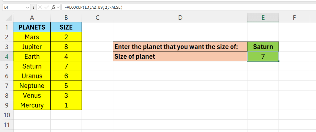
In below picture – we enter a name of a planet – and as a result we get its size.

Our formula will go in cell E4.

=VLOOKUP(E3;A2:B9;2;FALSE)

Above, E3 is the name of the planet we enter in cell E3.

The table array is where we get the information from – A2:B9

Finally we enter the column index – that is from column 2 – column B.