Excel tutorials

In the previous part we saw how we can get the highest value in a range using the =MAX() operation.

In this part we are going to output the location of the highest score in a given range.

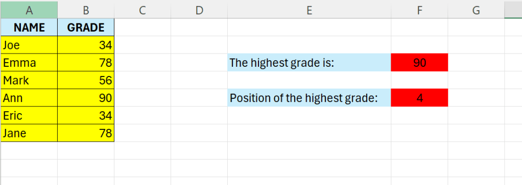
The final result are going to look like this:

For details regarding the MAX-function – see the previous post.

Here we are going to combine the =MATCH() function with the =MAX() function.

The syntax is as follows:

=MATCH(lookup_value,lookup_array,[match_type])

• lookup_value – The value to match in lookup_array
• lookup_array – A range of cells
• match_type – [optional] 1 = exact or next smallest (default), 0 = exact match, -1 = exact or next largest.

Now, in cell F5 enter the following formula:

=MATCH(MAX(B2:B8);B2:B8;0)

The MAX function returns the maximum value in the range, and the MATCH function returns the position of the maximum in the given range.