Excel tutorials

In Excel there are a lot of different ways to highlight duplicates, we can use formulas in a variety of ways or we can use conditional formatting. Here in this tutorials we are going to use one of the most simple ways to highlight duplicates in a range.

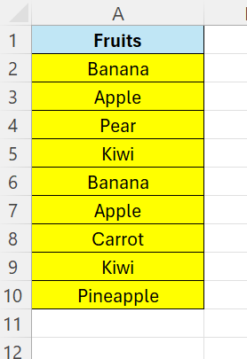
To illustrate this we start by adding some data in column A.

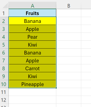
Now, select all the data that you want to search for duplicates. That is, select cell A2 to A10.

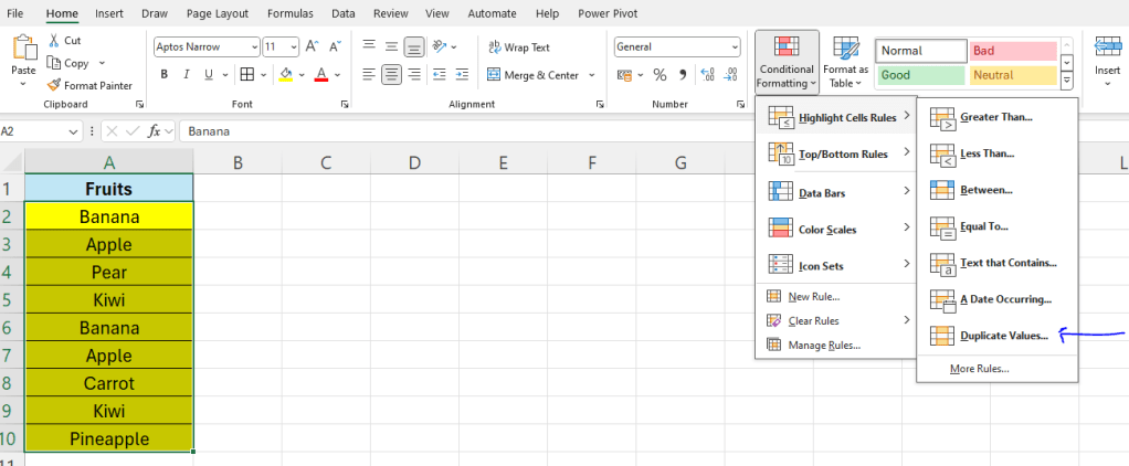
Next, on the Home tab – locate “Conditional Formatting” – then select “Highlight cell Rules” – then at the bottom, choose “Duplicate values“

A new window appear, here you can select colors etc, just click OK

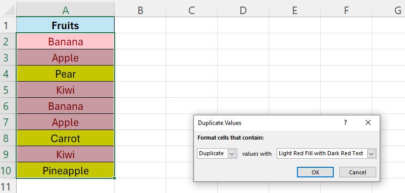
All duplicates now have a purple/red color.